How-to Guide 3: Conduct Monte Carlo Simulations and Sensitivity Analysis

Mimi includes a host of routines which support running Monte Carlo simulations and various sensitivity analysis methods on Mimi models. Tutorial 5: Monte Carlo Simulations and Sensitivity Analysis Support is a good starting point for learning about these methods. This how-to guide includes more detail and optionality, covering more advanced options such as non-stochastic scenarios and running multiple models, which are not yet included in the tutorial.

Overview

Running Monte Carlo simulations, and proximal sensitivity analysis, in Mimi can be broken down into three primary user-facing elements:

The @defsim macro, which defines random variables (RVs) which are assigned distributions and associated with model parameters, and override the default (random) sampling method.
The run function, which runs a simulation instance, setting the model(s) on which a simulation definition can be run within that, generates all trial data with generate_trials!, and has several with optional parameters and optional callback functions to customize simulation behavior.
The analyze function, which takes a simulation instance, analyzes the results and returns results specific to the type of simulation passed in.

The rest of this document will be organized as follows:

The @defsim macro
The run function
The analyze function
Plotting and the Explorer UI
Other Useful Functions
Examples

We will refer separately to two types, SimulationDef and SimulationInstance. They are referred to as sim_def and sim_inst respectively as function arguments, and sd and si respectively as local variables.

1. The `@defsim` macro

The first step in a Mimi sensitivity analysis is using the @defsim macro to define and return a SimulationDef{T}. This simulation definition contains all the definition information in a form that can be applied at run-time. The T in SimulationDef{T} is any type that your application would like to live inside the SimulationDef struct, and most importantly specifies the sampling strategy to be used in your sensitivity analysis.

We have implemented four types for T <: AbstractSimulationData:

Simple random-sampling Monte Carlo Simulation (MCSData),
Latin Hypercube Sampling (LHSData)
Sobol sampling and analysis (SobolData)
Delta sampling and analysis (DeltaData) - Beta, we don't recommend use yet

We also define type constants with friendlier names for these parameterized types:

const MonteCarloSimulationDef = SimulationDef{MCSData}
const MonteCarloSimulationInstance = SimulationInstance{MCSData}

const LatinHypercubeSimulationDef = SimulationDef{LHSData}
const LatinHypercubeSimulationInstance = SimulationInstance{LHSData}

const SobolSimulationDef = SimulationDef{SobolData}
const SobolSimulationInstance = SimulationInstance{SobolData}

const DeltaSimulationDef = SimulationDef{DeltaData}
const DeltaSimulationInstance = SimulationInstance{DeltaData}

In order to build the information required at run-time, the @defsim macro carries out several tasks including the following.

Define Random Variables (RVs)

The macro must define random variables (RVs) by assigning names to distributions, which can be any object that supports the following function:

rand(dist, count::Int=1) which produces a single value when count == 1, else a Vector of values.

If using Latin Hypercube Sampling (LHS) is used, the following function must also be defined:

quantile(dist, quantiles::Vector{Float64}) which returns values for the given quantiles of the distribution.

In addition to the distributions available in the Distributions package, Mimi provides the following options. Note that these are not exported by default, so they need to either be explicitly imported (ie. import Mimi: EmpiricalDistribution) or prefixed with Mimi. when implemented (ie. Mimi.EmpiricalDistribution(vals, probs)):

EmpiricalDistribution, which takes a vector of values and (optional) vector of probabilities and produces samples from these values using the given probabilities, if provided, or equal probability otherwise. To use this in a @defsim, you might do:

using CSVFiles
using DataFrames
using Mimi
import Mimi: EmpiricalDistribution # not currently exported so you just need to grab it

# read in your values
values = load("path_to_values_file"; header_exists = false) |> DataFrame
# read in your probabilities (optional, if none are provided we assume all equal)
# note that the probabilities need to be Float type and should roughly add to 1
probs = load("path_to_probabilities_file"; header_exists = false) |> DataFrame

# create your simulation
@defsim  begin
    ...
    RandomVariable1 = EmpiricalDistribution(values, probs)
    ...
end

Note there are many ways to load values, we use DataFrames and CSVFiles above but there might be an easier way depending on what packages you like

SampleStore{T}, which stores a vector of samples that are produced in order by the rand function. This allows the user to to store a predefined set of values (useful for regression testing) and it is used by the LHS method, which draws all required samples at once at equal probability intervals and then shuffles the values. It is also used when rank correlations are specified, since this requires re-ordering draws from random variables.
ReshapedDistribution, which supports use of vector-valued distributions, i.e., those that generate vectors of values for each single draw. An example (that motivated this addition) is the Dirichlet distribution, which produces a vector of values that sum to 1. To use this in @defsim, you might do:
```
  rd = ReshapedDistribution([5, 5], Dirichlet(25,1))
```
This code creates a pseudo-distribution that, for each draw, produces a 5x5 matrix of values that sum to 1.

Apply RVs to model parameters

For all applications in this section, it is important to note that for each trial, a random variable on the right hand side of an assignment will take on the value of a single draw from the given distribution. This means that even if the random variable is applied to more than one parameter on the left hand side (such as assigning to a slice), each of these parameters will be assigned the same value, not different draws from the distribution.

The macro next defines how to apply the values generated by each RV to model parameters based on a pseudo-assignment operator. The left hand side of these assignments can be either a param, which must refer to a shared model parameter, or comp.param which refers to an unshared model parameter specific to a component.

param = RV or comp.param = RV replaces the values in the parameter with the value of the RV for the current trial.
param += RV or comp.param += RV replaces the values in the parameter with the sum of the original value and the value of the RV for the current trial.
param *= RV or comp.param *= RV replaces the values in the parameter with the product of the original value and the value of the RV for the current trial.

As described below, in @defsim, you can apply distributions to specific slices of array parameters, and you can "bulk assign" distributions to elements of a vector or matrix using a more condensed syntax. Note that these relationship assignments are referred to as transforms, and are referred to later in this documentation in the add_transform! and delete_transform! helper functions.

Apply RVs to model parameters: Assigning to array slices

Options for applying distributions to array slices is accomplished using array access syntax on the left-hand side of an assignment. The assignment may use any of these assignment operators: =, *=, or +=, as described above. Slices can be indicated using a variety of specifications. Assume we define two parameters in @defcomp as

  foo = Parameter(index=[regions])
  bar = Parameter(index=[time, regions])

with regions defined as [:USA, :CAN, :MEX, :ROW]

We can assign distributions to the elements of foo several ways:

Using a symbol or string or tuple of symbols or strings. Note that values specified without a ":" prefix or double quotes are treated as symbols. To specify strings, quote them the usual way.
- foo[USA] = Uniform(0, 1) would assign the RV to foo[:USA] only.
- foo[(USA, CAN, MEX)] = Uniform(0, 1) would assign the same RV to 3 elements of foo. That is, a single value is drawn from the RV with distribution Uniform(0, 1) and this value is assigned to all three elements of foo.
A :, indicating all elements for this dimension
- foo[:] = Normal(10.0 3.0) would use a draw from the Normal RV for all elements of foo.
A : range, with or without a step, or a tuple of integers
- bar[2050:10:2080, :] = Uniform(2, 3) would assign a single Uniform RV to all regions for time steps with labels 2050, 2060, 2070, and 2080.
- bar[(2050, 2060, 2070, 2080), :] = Uniform(2, 3) does the same thing using a tuple of values.

If regions were defined using strings, as in ["USA", "CAN", "MEX", "ROW"], the examples above would be written as foo["USA"] = Uniform(0, 1) and so on.

Apply RVs to model parameters: Assigning a vector of distributions

In some cases, it's more convenient to assign a vector of distributions (e.g., with different functional forms or parameters) to a single parameter. For example we can use the following syntax:

  foo = [USA => Uniform(0, 1),
         (CAN, MEX) => Uniform(1, 2),
         ROW => Normal(10, 3)]

which is equivalent to:

  foo[USA] = Uniform(0, 1),
  foo[(CAN, MEX)] = Uniform(1, 2),
  foo[ROW] = Normal(10, 3)]

To assign to parameters with more than one dimension, use square brackets around the dimensions on the left-hand side of each => operator, e.g.,

  bar = [[2050, USA] => Uniform(0, 1),
         [:, (CAN, MEX)] => Uniform(1, 2),
         [2010:10:2080, ROW] => Normal(10, 3)]

Currently, the more condensed syntax (using the pair operator =>) supports only direct assignment of RV value, i.e., you cannot combine this with the *= or += operators.

Specify a Sampling Strategies

As previously mentioned and included in the tutorial, the @defsim macro uses the call to sampling to type-parameterize the SimulationDef with one of three types, which in turn direct the sampling strategy of the simulation. This is done with the sampling line of the macro.

Simple random-sampling Monte Carlo Simulation (MCSData),
Latin Hypercube Sampling (LHSData)

Latin Hypercube sampling divides the distribution into equally-spaced quantiles, obtains values at those quantiles, and then shuffles the values. The result is better representation of the tails of the distribution with fewer samples than would be required for purely random sampling.

Sobol sampling and analysis (SobolData)
Delta sampling and analysis (DeltaData) - Beta, we don't recommend use yet

Include Sampling Strategy-specific Parameters

Certain sampling strategies support (or necessitate) further customization. These may include:

rank correlations (LHS)): In some cases, it may be desireable to define rank correlations between pairs of random variables. Approximate rank correlation is achieved by re-ordering vectors of random draws as per Iman and Conover (1982).
extra parameters (Sobol): Sobol sampling allows specification of the sample size N and whether or not one wishes to calculate second-order effects.

2. The `run` function

In it's simplest use, the run function generates and iterates over generated trial data, perturbing a chosen subset of Mimi's model parameters, based on the defined distributions, and then runs the given Mimi model(s). The function retuns an instance of SimulationInstance, holding a copy of the original SimulationDef with additional trial information as well as a list of references ot the models and the results. Optionally, trial values and/or model results are saved to CSV files.

Function signature

The full signature for the run is:

function Base.run(sim_def::SimulationDef{T}, models::Union{Vector{Model}, Model}, samplesize::Int;
                 ntimesteps::Int=typemax(Int), 
                 trials_output_filename::Union{Nothing, AbstractString}=nothing, 
                 results_output_dir::Union{Nothing, AbstractString}=nothing, 
                 pre_trial_func::Union{Nothing, Function}=nothing, 
                 post_trial_func::Union{Nothing, Function}=nothing,
                 scenario_func::Union{Nothing, Function}=nothing,
                 scenario_placement::ScenarioLoopPlacement=OUTER,
                 scenario_args=nothing,
                 results_in_memory::Bool=true) where T <: AbstractSimulationData

Using this function allows a user to run the simulation definition sim_def for the models using samplesize samples.

Optionally the user may run the models for ntimesteps, if specified, else to the maximum defined time period. Note that trial data are applied to all the associated models even when running only a portion of them.

If provided, the generated trials and results will be saved in the indicated trials_output_filename and results_output_dir respectively. If results_in_memory is set to false, then results will be cleared from memory and only stored in the results_output_dir. After run, the results of a SimulationInstance can be accessed using the getdataframe function with the following signature, which returns a DataFrame.

getdataframe(sim_inst::SimulationInstance, comp_name::Symbol, datum_name::Symbol; model::Int = 1)

If pre_trial_func or post_trial_func are defined, the designated functions are called just before or after (respectively) running a trial. The functions must have the signature:

fn(sim_inst::SimulationInstance, trialnum::Int, ntimesteps::Int, tup::Tuple)

where tup is a tuple of scenario arguments representing one element in the cross-product of all scenario value vectors. In situations in which you want the simulation loop to run only some of the models, the remainder of the runs can be handled using a pre_trial_func or post_trial_func.

If provided, scenario_args must be a Vector{Pair}, where each Pair is a symbol and a Vector of arbitrary values that will be meaningful to scenario_func, which must have the signature:

scenario_func(sim_inst::SimulationInstance, tup::Tuple)

By default, the scenario loop encloses the simulation loop, but the scenario loop can be placed inside the simulation loop by specifying scenario_placement=INNER. When INNER is specified, the scenario_func is called after any pre_trial_func but before the model is run.

Finally, run returns the type SimulationInstance that contains a copy of the original SimulationDef in addition to trials information (trials, current_trial, and current_data), the model list models, and results information in results.

Internal Functions to `run`

The following functions are internal to run, and do not need to be understood by users but may be interesting to understand.

The set_models! function

The run function sets the model or models to run using set_models! function and saving references to these in the SimulationInstance instance. The set_models! function has several methods for associating the model(s) to run with the SimulationDef:

set_models!(sim_inst::SimulationInstance, models::Vector{Model})
set_models!(sim_inst::SimulationInstance, m::Model)
set_models!(sim_inst::SimulationInstance, mm::MarginalModel)

The generate_trials! function

The generate_trials! function is used to pre-generate data using the given samplesize and save all random variable values in the file filename. Its calling signature is:

  generate_trials!(sim_def::SimulationDefinition, samplesize::Int; filename::Union{String, Nothing}=nothing)

If the sim_def parameter has multiple scenarios and the scenario_loop placement is set to OUTER this function must be called if the user wants to ensure the same trial data be used in each scenario. If this function is not called, new trial data will be generated for each scenario.

Also note that if the filename argument is used, all random variable draws are saved to the given filename. Internally, any Distribution instance is converted to a SampleStore and the values are subsequently returned in the order generated when rand! is called.

Non-stochastic Scenarios

In many cases, scenarios (which we define as a choice of values from a discrete set for one or more parameters) need to be considered in addition to the stochastic parameter variation. To support scenarios, run also offers iteration over discrete scenario values, which are passed to run via the keyword parameter scenario_args::Dict{Symbol, Vector}. For example, to iterate over scenario values "a", and "b", as well as, say, discount rates 0.025, 0.05, 0.07, you could provide the argument:

scenario_args=Dict([:name => ["a", "b"], :rate => [0.025, 0.05, 0.07]])

Of course, the SA subsystem does not know what you want to do with these values, so the user must also provide a callback function in the scenario_func argument. This function must be defined with the signature:

function any_name_you_like(sim_inst::SimulationInstance, tup)

where tup is an element of the set of tuples produced by calling Itertools.product() on all the scenario arguments. In the example above, this would produce the following vector of tuples:

[("a", 0.025), ("b", 0.025), ("a", 0.03), ("b", 0.03), ("a", 0.05), ("b", 0.05)].

This approach allows all scenario combinations to be iterated over using a single loop. A final keyword argument, scenario_placement::ScenarioLoopPlacement indicates whether the scenario loop should occur inside or outside the loop over stochastic trial values. The type ScenarioLoopPlacement is an enum with values INNER and OUTER, the latter being the default placement.

In approximate pseudo-julia, these options produce the following behavior:

scenario_placement=OUTER

for tup in scenario_tuples
  scenario_func(tup)

  # for each scenario, run all SA trials
  for trial in trials
    trial_data = get_trial_data(trial)
    apply_trial_data()

    pre_trial_func()
    run(model)
    post_trial_func()
  end
end

scenario_placement=INNER

for trial in trials
  trial_data = get_trial_data(trial)
  apply_trial_data()

  # for each SA trial, run all scenarios
  for tup in scenario_tuples
    scenario_func(tup)

    pre_trial_func()
    run(model)
    post_trial_func()
  end
end

Running Multiple Models

In some simulations, a baseline model needs to be compared to one or more models that are perturbed parametrically or structurally (i.e., with different components or equations.) To support this, the SimulationInstance type holds a vector of Model instances, and allows the caller to specify how many of these to run automatically for each trial. Note that regardless of how many models are run, the random variables are applied to all of the models associated with the simulation.

By default, all defined models are run. In some cases, you may want to run some of the models "manually" in the pre_trial_func or post_trial_func, which allow you to make arbitrary modifications to these additional models.

3. The `analyze` function

The analyze function takes a simulation instance, runs a sensitivity analysis method as determined by the type of simulation instance, and returns the results. It is currently defined for a SobolSimulationInstance and the DeltaSimulationInstance (Beta) subtypes of SimulationInstance.

This function wraps the analyze function in the GlobalSensitivityAnalysis.jl package, so please view the README of this package for the most up to date information.

4. Plotting and the Explorer UI

As described in the User Guide, Mimi provides support for plotting using VegaLite and VegaLite.jl within the Mimi Explorer UI and Mimi.plot function. These functions not only work for Models, but for SimulationInstances as well.

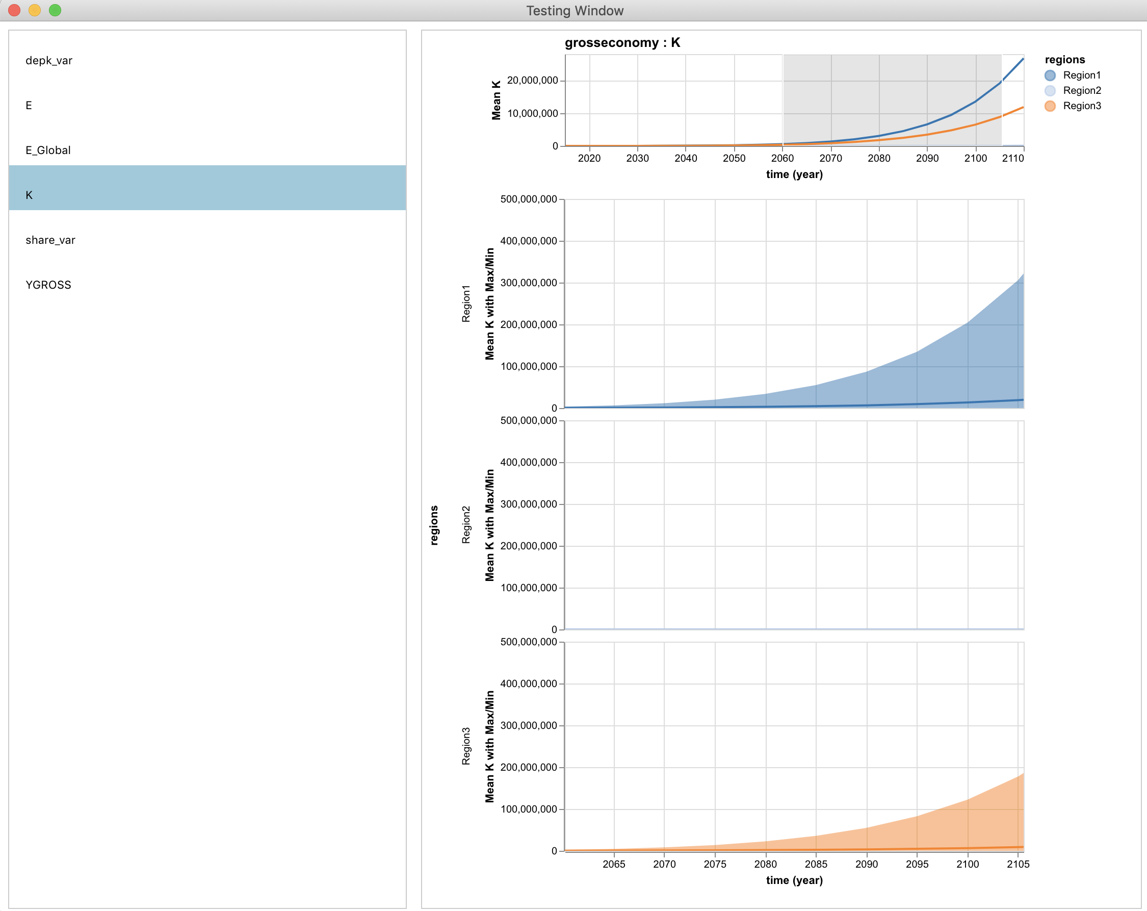
In order to invoke the explorer UI and explore all of the saved variables from the save list of a SimulationInstance, simply call the function explore with the simulation as the required argument as shown below. This will produce a new browser window containing a selectable list of variables, each of which produces a graphic.

run(sim_inst)
explore(sim_inst)

There are several optional keyword arguments for the explore method, as shown by the full function signature:

explore(sim_inst::SimulationInstance; title="Electron", model_index::Int = 1, scen_name::Union{Nothing, String} = nothing, results_output_dir::Union{Nothing, String} = nothing)

The title is the optional title of the application window, the model_index defines which model in your list of models passed to run you would like to explore (defaults to 1), and scen_name is the name of the specific scenario you would like to explore if there is a scenario dimension to your simulation. Note that if there are multiple scenarios, this is a required argument. Finally, if you have saved the results of your simulation to disk and cleared them from memory using run's results_in_memory keyword argument flag set to false, you must provide a results_output_dir which indicates the parent folder for all outputs and potential subdirectories, identical to that passed to run.

Explorer Simulation Example

Alternatively, in order to view just one variable, call the (unexported) function Mimi.plot as below to return a plot object and automatically display the plot in a viewer, assuming Mimi.plot is the last command executed. Note that plot is not exported in order to avoid namespace conflicts, but a user may import it if desired. This call will return the type VegaLite.VLSpec, which you may interact with using the API described in the VegaLite.jl documentation. For example, VegaLite.jl plots can be saved in many typical file formats such as PNG, SVG, PDF and EPS files. You may save a plot using the save function. Note that while explore(sim_inst) returns interactive plots for several graphs, Mimi.plot(si, :foo, :bar) will return only static plots.

using VegaLite
run(sim_inst)
p = Mimi.plot(sim_inst, :component1, :parameter1)
save("figure.svg", p)

Note the function signature below, which has the same keyword arguments and requirements as the aforementioned explore method, save for title.

plot(sim_inst::SimulationInstance, comp_name::Symbol, datum_name::Symbol; interactive::Bool = false, model_index::Int = 1, scen_name::Union{Nothing, String} = nothing, results_output_dir::Union{Nothing, String} = nothing)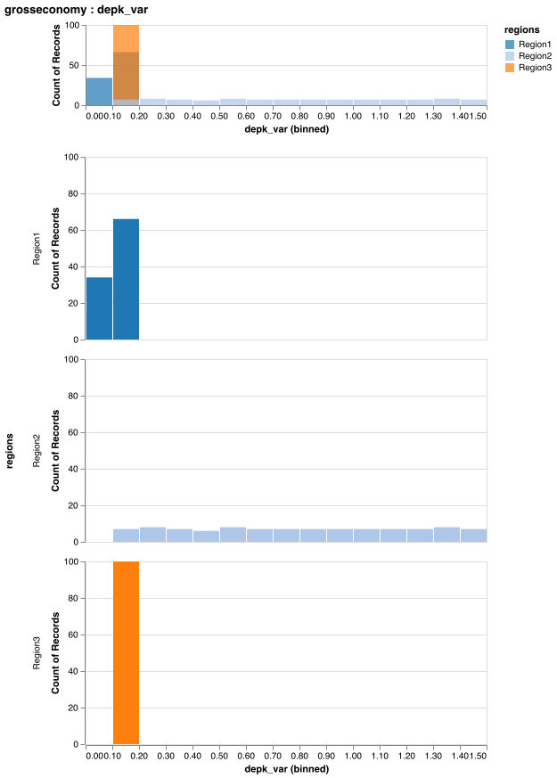

Plot Simulation Example

5. Other Useful Functions

Simulation Modification Functions

A small set of unexported functions are available to modify an existing SimulationDefinition. The functions include:

delete_RV!(sim_def::SimulationDef, name::Symbol) - deletes the random variable with name name from the Simulation Definition sim_def, along with all transformations using that random variable
add_RV!(sim_def::SimulationDef, name::Symbol, dist::Distribution) - add the random variable with the name name from the Simulation Definition sim_def
replace_RV!(sim_def::SimulationDef, name::Symbol, dist::Distribution) - replace the random variable with name name in Simulation Definition with a random variable of the same name but with the distribution Distribution
delete_transform!(sim_def::SimulationDef, name::Symbol)! - Delete all data transformations in Simulation Definition sim_def (i.e., replacement, addition or multiplication) of original data values with values drawn from the random variable named name
add_transform!(sim_def::SimulationDef, paramname::Symbol, op::Symbol, rvname::Symbol, dims::Vector=[])! - Create a new TransformSpec based on paramname, op, rvname and dims to the Simulation Definition sim_def. The symbol rvname must refer to an existing random variable, and paramname must refer to an existing shared model parameter that can thus be accessed by that name. Use the following signature if your paramname is an unshared model parameter specific to a component. If dims are provided, these must be legal subscripts of paramname. Op must be one of :+=, :*=, or :(=).
add_transform!(sim_def::SimulationDef, compname::Symbol, paramname::Symbol, op::Symbol, rvname::Symbol, dims::Vector=[])! - Create a new TransformSpec based on compname, paramname, op, rvname and dims to the Simulation definition sim_def, and update the Simulation's NamedTuple type. The symbol rvname must refer to an existing RV, and compname and paramname must holding an existing component and parameter. If dims are provided, these must be legal subscripts of paramname. Op must be one of :+=, :*=, or :(=).

For example, say a user starts off with a SimulationDefinition MySimDef with a parameter MyParameter drawn from the random variable MyRV with distribution Uniform(0,1).

Case 1: The user wants this random variable to draw from a new distribution, say Normal(0,1), which will affect all parameters with transforms attached to this random variable.

using Distributions
using Mimi
replace_RV!(MySimDef, MyRV, Normal(0,1))

Case 2: The user parameter MyParameter to to take on the value of a random draw from a Normal(2,0.1) distribution. We assume this requires a new random variable, because no random variable has this distribution yet.

using Distributions
using Mimi
add_RV!(MySimDef, :NewRV, Normal(2, 0.1))
add_transform!(MySimDef, :MyParameter, :=, :NewRV)

add_save!(sim_def::SimulationDef, comp_name::Symbol, datum_name::Symbol) - Add to Simulation Definitionsim_def a "save" instruction for component comp_name and parameter or variable datum_name. This result will be saved to a CSV file at the end of the simulation.
delete_save!(sim_def::SimulationDef, comp_name::Symbol, datum_name::Symbol) - Delete from Simulation Definition sim_def a "save" instruction for component comp_name and parameter nor variable datum_name. This result will no longer be saved to a CSV file at the end of the simulation.

Helper Functions

"""
  get_simdef_rvnames(sim_def::SimulationDef, name::Union{String, Symbol})

A helper function to support finding the keys in a Simulation Definition `sim_def`'s
rvdict that contain a given `name`. This can be particularly helpful if the random 
variable was set via the shortcut syntax ie. my_parameter = Normal(0,1) and thus the
`sim_def` has automatically created a key in the format `:my_parameter!x`. In this 
case this function is useful to get the key and carry out modification functions 
such as `replace_rv!`.
"""

function get_simdef_rvnames(sim_def::SimulationDef, name::Union{String, Symbol})
    names = String.([keys(sim_def.rvdict)...])
    matches = Symbol.(filter(x -> occursin(String(name), x), names))
end

As shown in the examples below, and described above, parameters can be assigned unique random variables under the hood without explicitly declaring the RV. Fore example, instead of pairing

rv(name) = Uniform(0.2, 0.8)
share = name1

we can write

share = Uniform(0.2, 0.8)

When this is done, Mimi will create a new unique RV with a unique name share!x where x is an integer determined by internal processes that gaurantee it to be unique in this sim_def. This syntax is therefore not recommended if the user expects to want to reference that random variable using the aforementioned modification functions. That said, if the user does need to do so we have added a helper function get_simdef_rvnames(sim_def::SimulationDef, name::Union{String, Symbol}) which will return the unique names of the random variables that start with name. In the case above, for example, get_simdef_rvnames(sim_def, :share) would return [share!x]. In a case where share had multiple dimensions, like three regions, it would return [share!x1, share!x2, share!x3].

Payload Functions

set_payload!
payload

6. Examples

The following example is derived from "Mimi.jl/test/mcs/test_defmcs.jl".

using Mimi
using Distributions

N = 100

sd = @defsim begin
    # Define random variables. The rv() is required to disambiguate an
    # RV definition name = Dist(args...) from application of a distribution
    # to a model parameter. This makes the (less common) naming of an
    # RV slightly more burdensome, but it's only required when defining
    # correlations or sharing an RV across parameters.
    rv(name1) = Normal(1, 0.2)
    rv(name2) = Uniform(0.75, 1.25)
    rv(name3) = LogNormal(20, 4)

    # assign RVs to model Parameters
    share = Uniform(0.2, 0.8)
    sigma[:, Region1] *= name2
    sigma[2020:5:2050, (Region2, Region3)] *= Uniform(0.8, 1.2)

    depk = [Region1 => Uniform(0.08, 0.14),
            Region2 => Uniform(0.10, 1.50),
            Region3 => Uniform(0.10, 0.20)]

    sampling(LHSData, corrlist=[(:name1, :name2, 0.7), (:name1, :name3, 0.5)])
    
    # indicate which parameters to save for each model run. Specify
    # a parameter name or [later] some slice of its data, similar to the
    # assignment of RVs, above.
    save(grosseconomy.K, grosseconomy.YGROSS, emissions.E, emissions.E_Global)
end

Mimi.reset_compdefs()
include("../../examples/tutorial/02-multi-region-model/main.jl")

m = model

# Optionally, user functions can be called just before or after a trial is run
function print_result(m::Model, sim_inst::SimulationInstance, trialnum::Int)
    ci = Mimi.compinstance(m.mi, :emissions)
    value = Mimi.get_variable_value(ci, :E_Global)
    println("$(ci.comp_id).E_Global: $value")
end

# set some some constants
trials_output_filename = joinpath(output_dir, "trialdata.csv")
results_output_dir = joinpath(tempdir(), "sim")
N = 100

# Run trials and save trials results to the indicated directories
si = run(sd, m, N; trials_output_filename=trials_output_filename, results_output_dir=results_output_dir)

# take a look at the results
results = getdataframe(si, :grosseconomy, :K) # model index chosen defaults to 1

2. The run function

2. The `run` function